Autonomous Robots - Probability
- Motivation
- Discrete Probability Distributions
- Continuous Probability Distributions
- Bayes Theorem
- Gaussian Distribution
Motivation
 – Delivery Robots
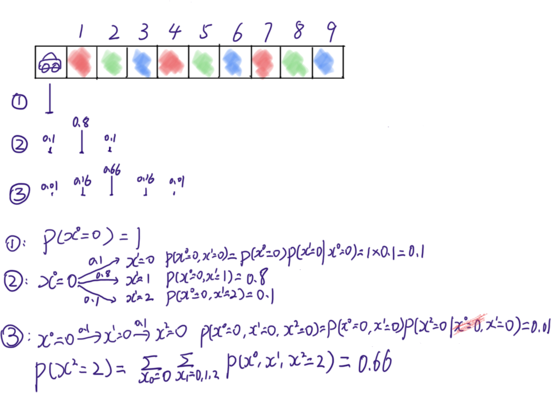
We have a delivery robot moving in one dimensional space. At $t = 0$, the robot is at $x^{t=0} = 0$, i.e. $p(x^0 = 0) = 1$. We can command robot to move forward a step at a time. However, it is possible that the robot stays at the same cell ($p(stay) = 0.1$), or steps into the next cell ($p(next) = 0.8$), or steps into the next next cell ($p(next_next) = 0.1$).
Pop Quiz: How likely the robot is in $x^{t=2} = 2$ at $t=2$, i.e. what is $p(x^{t=2}=2)$?

 $p(x^{t=1}=1) = 0.8$ and
$p(x^{t=2}=2) = 0.66$.
The robot gets more and more uncertain about its location as it moves.
$p(x^{t=1}=1) = 0.8$ and
$p(x^{t=2}=2) = 0.66$.
The robot gets more and more uncertain about its location as it moves.
We calculate $p(x^{t=2}=2)$ using the equation below. It uses Marginalization, Conditioning, etc. Though we will get into these into details in this post, I would like to show you an alternative way so called particle filtering or Monte Carlo Simulation.
\[\sum_{x^{t=0}=0}{\sum_{x^{t=1}=0,1,2}{p(x^{t=0}, x^{t=1}, x^{t=2}=2)}}\]
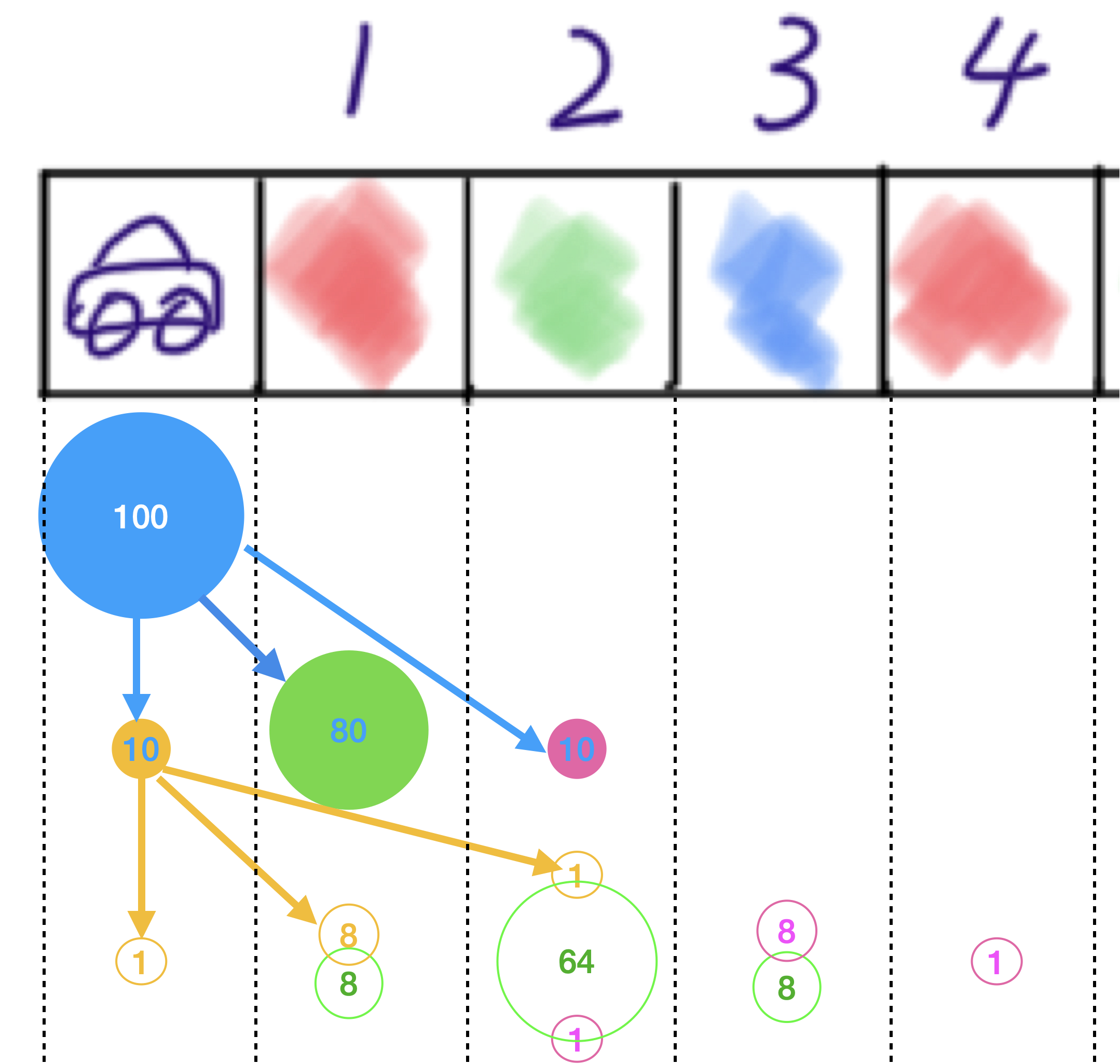
Suppose we have $100$ robots sitting at $x^{t=0} = 0$, then if when they all move forward one step, we will have $10$ robots stay at $x^{t=1}=0$, i.e. $N(x^{t=1}=0)=10$. Similarly, we can get $N(x^{t=1}=1)=80$ and $N(x^{t=1}=2)=10$. Then if all robots move one step forward again. $64$ robots out of $N(x^{t=1}=1)=80$ will be at $x^{t=2}=2$, $1$ robot out of $N(x^{t=1}=0)=10$ will be at $x^{t=2}=2$, and $1$ robot out of $N(x^{t=1}=2)=10$ will be at $x^{t=2}=2$. So total number of robots at $N(x^{t=2})=64+1+1=66$, and we have $p(x^{t=2}=2) = 0.66$.
Apparently, we can’t really rely on control commands to send robot to a target location because robots get more and more uncertain about its position. The solution is adding a sensor to the robot to sense the cell color.
Pop Quiz: If the sensor only detects the color correctly 80% time, and mis-detects the color as the other two 10% time respectively. How can we update the robot location distribution based on observations? For example, if at $t=2$, the robot observes cell color as blue, then what is $p(x^{t=2}=2)$ and $p(x^{t=2}=3)$?
Discrete Probability Distributions
– Probability Rules
-
$\sum_i{P(i)} = 1$
-
$0 \leq P(i) \leq 1$
-
$E[X] = \sum_x{xp(x)}$
-
$COV[X, Y] = E[(X-E[X])(Y-E[Y])]$
– Marginalization and Conditioning
- $P(Y) = \sum_i{P(X=x_i,Y)}$
- $P(X|Y=y_i)$
Pop Quiz: We have a joint probability distribution that encodes the relation between vehicles turning right and turning on right-turn signal at an intersection shown below. How likely a car will go straight (marginalization)? How likely a car will turn on the turn signal if it turns right (conditioning)?
\[P(turn-right,\ on) = 0.2\]
\[P(turn-right,\ off) = 0.2\]
\[P(go-straight,\ on) = 0.01\]
\[P(go-straight,\ off) = 0.59\]
Continuous Probability Distributions
– Probability Rules
-
$\int{p(x)}dx = 1$
-
$0 \leq p(x)$
-
$E[X] = \int{xp(x)}dx$
-
$COV[X, Y] = E[(X-E[X])(Y-E[Y])]$
– Marginalization and Conditioning
- $P(Y) = \int{P(X,Y)}dX$
- $P(X|Y=y_i)$
Bayes Theorem
– Basic Rule
\[P(X|Y) = \frac{P(Y|X)P(X)}{P(Y)}\]
– Joint Probability
\[P(X_1, \cdots, X_n) = P(X_1)P(X_2|X_1)P(X_3|X_2,X_1) \cdots P(X_n|X_{n-1}, X_{n-2},\cdots,X_1)\]
– First Order Markov Chain
\[P(X_1, \cdots, X_n) = P(X_1)P(X_2|X_1)P(X_3|X_2) \cdots P(X_n|X_{n-1})\]
The delivery robot example
is using first-order markov chain and marginalization:
\[P(x^{t=T}) = \sum_{x^{t=0},\cdots, x^{t=T-1}}{P(x^{t=0}, \cdots, x^{t=T})} = P(x^{t=0})P(x^{t=2}|x^{t=0}) \cdots\]
– Recursive Bayesian Estimation
\[p(x_k | u_0, \cdots, u_k, z_0, \cdots, z_k) = \frac{p(z_k , x_k | u_0, \cdots, u_k, z_0, \cdots, z_{k-1})}{p(z_k|u_0, \cdots, u_k, z_0, \cdots, z_{k-1})} \\ = \frac{p(z_k | x_k, u_0, \cdots, u_k, z_0, \cdots, z_{k-1}) \int{p(x_k, x_{k-1}| u_0, \cdots, u_k, z_0, \cdots, z_{k-1})}dx_{x-1}}{p(z_k|u_0, \cdots, u_k, z_0, \cdots, z_{k-1})} \\ = \frac{p(z_k | x_k) \int{p(x_k | x_{k-1}, u_0, \cdots, u_k, z_0, \cdots, z_{k-1})p(x_{k-1}| u_0, \cdots, u_k, z_0, \cdots, z_{k-1})}dx_{x-1}}{p(z_k|u_0, \cdots, u_k, z_0, \cdots, z_{k-1})} \\ = \frac{p(z_k | x_k) \int{p(x_k | x_{k-1}, u_k) p(x_{k-1}| u_0, \cdots, u_{k-1}, z_0, \cdots, z_{k-1})}dx_{x-1}}{p(z_k|u_0, \cdots, u_k, z_0, \cdots, z_{k-1})}\]
$Bel(x_k) = p(x_k | u_0, \cdots, u_k, z_0, \cdots, z_k)$
\[Bel(x_k) \propto p(z_k | x_k) \int{p(x_k | x_{k-1}, u_k) Bel(x_{k-1})}dx_{k-1}\]
\[Bel(x_k) \propto p(z_k | x_k) \sum_{x_{k-1}}{p(x_k | x_{k-1}, u_k) Bel(x_{k-1})}\]
Gaussian Distribution
The delivery robot example is actually using so called histogram filtering and particle filtering. As you can see, probability update of histogram filtering is very tedious. It would be nice to have a more compact way to represent the distribution, and a easier way to update the distribution. In this section, we will discuss about Gaussian Distribution.
– Formula
- 1-Dimensional
\[P(x) = \frac{e^{-\frac{1}{2}(x-\mu)^2}}{\sqrt{(2\pi)}\sigma}\]
- N-Dimensional
\[P(\textbf{x} \in \mathbb{R}^N) = \frac{e^{-\frac{1}{2}(\textbf{x}-\mu)^T\Sigma^{-1}(\textbf{x}-\mu)}}{\sqrt{((2\pi)^k\|\Sigma\|}}\]
-
$E[X] = \mu$
- $COV[X,X] = \Sigma$
– Marginalization
\[p(\alpha, \beta) \sim \mathcal{N}(\begin{bmatrix}\mu_{\alpha} \\
\mu_{\beta}\end{bmatrix}, \begin{bmatrix}\Sigma_{\alpha \alpha},
\Sigma_{\alpha \beta} \\ \Sigma_{\beta \alpha}, \Sigma_{\beta \beta} \end{bmatrix})\]
\[p(\alpha) = \int{p(\alpha, \beta)}d\beta \ \sim \mathcal{N}(\mu_{\alpha}, \Sigma_{\alpha \alpha})\]
– Conditioning
\[p(\alpha, \beta) \sim \mathcal{N}(\begin{bmatrix}\mu_{\alpha} \\
\mu_{\beta}\end{bmatrix}, \begin{bmatrix}\Sigma_{\alpha \alpha},
\ \Sigma_{\alpha \beta} \\ \Sigma_{\beta \alpha}, \Sigma_{\beta \beta} \end{bmatrix})\]
\[p(\alpha|\beta) = \frac{p(\alpha, \beta)}{p(\beta)} \ \sim \mathcal{N}(\mu_{\alpha} + \Sigma_{\alpha
\beta}\Sigma_{\beta \beta}^{-1}(\beta - \mu_{\beta}),\ \Sigma_{\alpha \alpha} - \Sigma_{\alpha\beta}\Sigma_{\beta\beta}^{-1}\Sigma_{\beta\alpha})\]
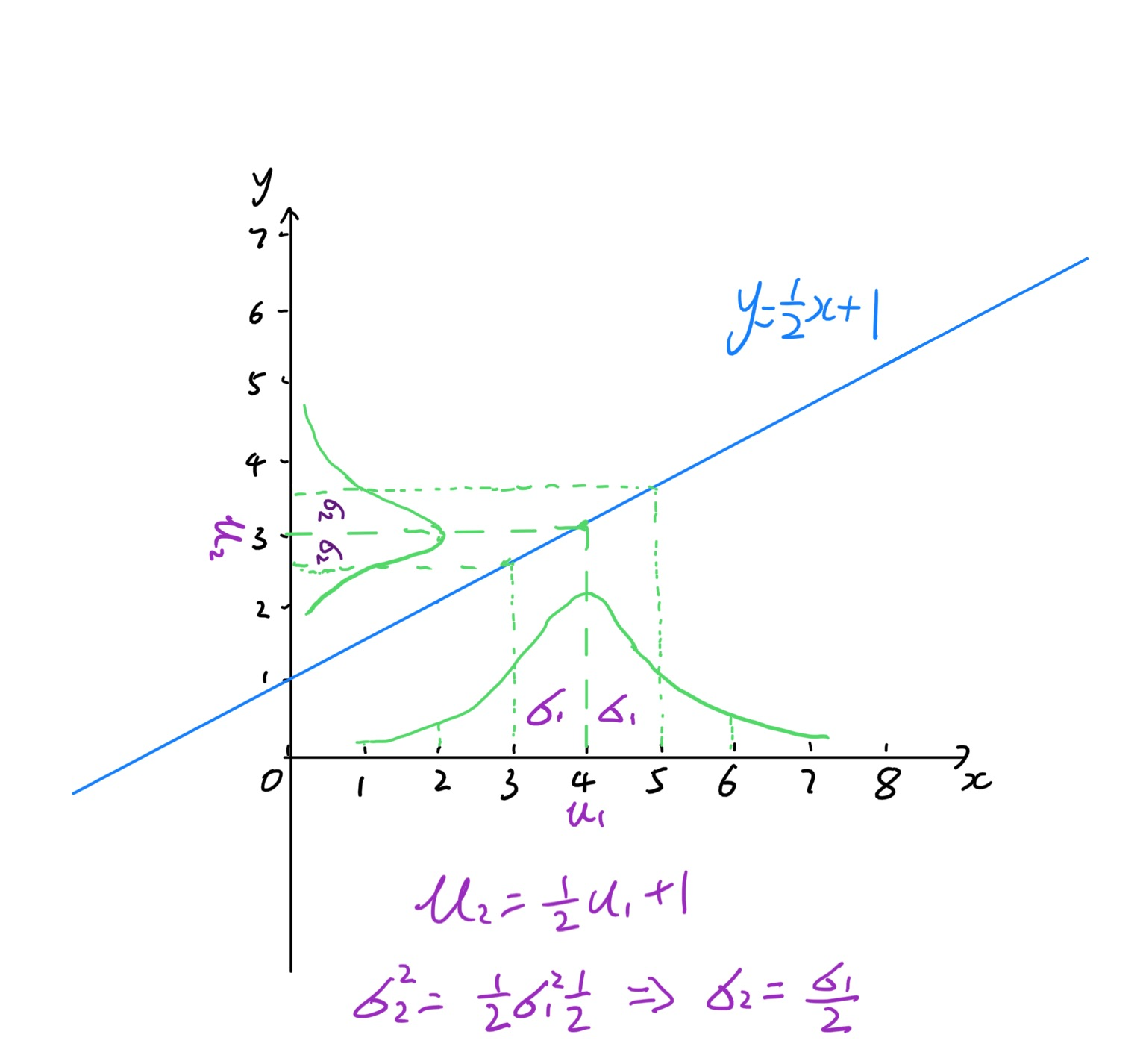
– Covariance Projection
Suppose we have $\textbf{x}
\sim \mathcal{N}(\mu_{x}, \Sigma_{xx})$ and $\textbf{y} = A\textbf{x} +
\textbf{b}$, then
\[\textbf{x} \sim \mathcal{N}(A\mu_{x}+\textbf{b}, A\Sigma_{xx}A^T)\]
The figure below shows the covariance projection of a 1-D Gaussian. To learn more
about proofs, check this
 .
.
Pop Quiz: If you can sample from a normal distribution $\textbf{x} \sim \mathcal{N}(\mu_{0}, I)$, how do you get samples from a Gaussian distribution $\textbf{x} \sim \mathcal{N}(\mu_{x}, \Sigma_{xx})$ ?
– Information Form
\(\textbf{x} \sim \mathcal{N}^{-1}(\eta, \Lambda)\) where $\eta = \Sigma^{-1}\mu$, $\Lambda = \Sigma^{-1}$
To learn more about marginalization and conditioning of information form, check this post.