Autonomous Robots - Linear Algebra
This post only covers I guess a minimal number of subjects of Linear Algebra required for autonomous robots. I might add more staff later.
Motivation
Let me motivate you with two examples.
 – GPS localization
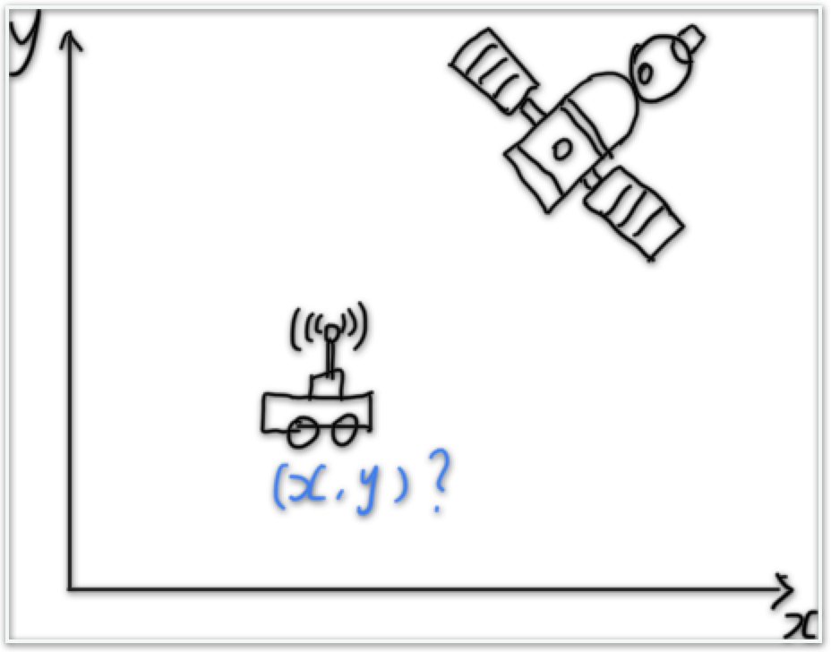
There is a GPS receiver on your robot, it can get robot’s $x$ and $y$ positions at 1HZ, i.e. $x_o^{t_0}, y_o^{t_0}, \cdots, x_o^{t_n}, y_o^{t_n}$. Because there are noises, so even the robot doesn’t move, it will not get exactly the same observations. Suppose you get $n$ observations, how do you figure out the best guess of your robot position? You probably think this is simple – use average. But let’s formulate it using Linear Algebra!

If you only have one pair of observations, then you will have two equations like this:
\[x = x_o^{t_0} \\ y = y_o^{t_0}\]
If you have two pairs of observations, then you will have four equations like this:
\[x = x_o^{t_0} \\ y = y_o^{t_0} \\ x = x_o^{t_1} \\ y = y_o^{t_1}\]
If you have $n$ pairs of observations, then you ill have $2n$ equation like this:
\[x = x_o^{t_0} \\ y = y_o^{t_0} \\ \vdots \\ x = x_o^{t_n} \\ y = y_o^{t_n}\]
Then we can write it into a matrix form and solve it.
\[\begin{bmatrix} 1, 0 \\ 0, 1 \\ \vdots, \vdots \\ 1, 0 \\ 0, 1 \end{bmatrix} \begin{bmatrix} x \\ y \end{bmatrix} = \begin{bmatrix} x_o^{t_0} \\ y_o^{t_0} \\ \vdots \\ x_o^{t_n} \\ x_o^{t_n} \end{bmatrix}\]
 – Line fitting
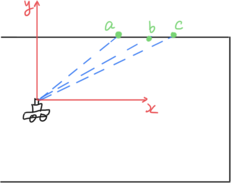
There is a Lidar on your robot. It sends out three beams $a, b, c$ and get the range between Lidar and the wall $r_a, r_b, r_c$. If the beam angle is known, we can end points positions $x_a, y_a, y_b, y_b, x_c, y_c$. So how do we fit a line using three points given the fact that a 2D line only has 2 degree of freedom.
Why do we need to fit a line? You will have a more compact representation of the world than using raw points.

Suppose we parameterize a 2D line as $y = \lambda x + \rho$, then
\[y_a = \lambda x_a + \rho \\ y_b = \lambda x_b + \rho \\ y_c = \lambda x_c + \rho\]
Pop Quiz: How many observations? How many unknowns?
Write the equations in matrix form:
\[\begin{bmatrix} x_a, 1 \\ x_b, 1 \\ x_c, 1 \end{bmatrix} \begin{bmatrix} \lambda \\ \rho \end{bmatrix} = \begin{bmatrix} y_a \\ y_b \\ y_c \end{bmatrix}\]
Vectors
 – Vector Representations
A two-dimensional vector $\textbf{v} \in \mathbb{R}^2$ can be written as a column vector:
\[\textbf{v} = \begin{bmatrix} v_1 \\ v_2 \end{bmatrix}\]
It can represent:
- direction and magnitude, e.g. the velocity of a point on a robot
- position, e.g. the position of a point on a robot
 – Vector Operations
- Scaling
$\lambda \textbf{v}$
- Linear combinations
$\alpha\textbf{v} + \beta\textbf{w}$
- Dot product
$\textbf{v}.dot(\textbf{w}) = \textbf{v}^T \textbf{w} = v_1w_1+\cdots+v_nw_n$, where $v,w \in \mathbb{R}^n$ $|\textbf{v}.dot(\textbf{w})| = |\textbf{v}||\textbf{w}|cos(\theta)$, where $\theta$ is the angle between two vectors.
- Cross product of vectors in $\mathbb{R}^3$
\(\textbf{v}.cross(\textbf{w}) = \begin{bmatrix} 0, -v_3, v_2\\ v_3, 0, -v_1 \\ -v_2, v_1, 0 \end{bmatrix} \begin{bmatrix} w_1 \\ w_2 \\ w_3 \\ \end{bmatrix}\) $|\textbf{v}.cross(\textbf{w})| = |\textbf{v}||\textbf{w}|sin(\theta)$, where $\theta$ is the angle between two vectors.
 – Examples of Vectors Operations in Robotics
-
Scaling
Starting at $O$, robot moves at a constant speed $\textbf{v}$. After $\Delta t$, the robot will be at $O + {\Delta t}\textbf{v}$
-
Linear combinations
Starting at $O \in \mathbb{R}^2$, robot moves at a constant speed $\dot{x} = \textbf{v}$ in $x$ direction and $\dot{y} = \textbf{w}$ in $y$ direction. After $\Delta t$, the robot will be at $O + {\Delta t}\textbf{v} + {\Delta t}\textbf{w}$
-
Dot product
Find two lines seen from the robot are parallel or not. If so, $1 = cos(\theta) = \frac{|\textbf{v}.dot(\textbf{w})|}{|\textbf{v}||\textbf{w}|}$
Pop quiz: How can you figure whether a point is inside a rectangle or not?
-
Cross product of vectors in $\mathbb{R}^3$
$v = \omega.cross(R)$, where $v$ is the linear velocity and $\omega$ is the angular velocity
Pop quiz: Find the shortest distance from a point to a line.
Matrices and Linear Equations
 – Matrix Representations
A $2 \times 2$ matrix can be written as a collection of two column vector $\textbf{v} \in \mathbb{R}^2$, $\textbf{w} \in \mathbb{R}^2$:
\[\begin{bmatrix} a_{11}, a_{12} \\ a_{21}, a_{22} \end{bmatrix} = \begin{bmatrix} \textbf{v}, \textbf{w} \end{bmatrix}\]
Similarly, a $3 \times 3$ matrix can be written as a collection of three column vector $\textbf{u} \in \mathbb{R}^3$, $\textbf{v} \in \mathbb{R}^3$, $\textbf{w} \in \mathbb{R}^3$:
\[\begin{bmatrix} a_{11}, a_{12}, a_{13} \\ a_{21}, a_{22}, a_{23} \\ a_{31}, a_{32}, a_{33} \end{bmatrix} = \begin{bmatrix} \textbf{u}, \textbf{v}, \textbf{w} \end{bmatrix}\]
 In this post, we will only
discuss about $m \times m$ matrix. Without considering numerical issues, knowing
properties of $m \times m$ is enough for us solving all kinds of linear
equations.
 – Matrix Operations
- Matrix multiplication
$C_{mm} = A_{mn}B_{nm}$
- Matrix times vector as a linear combination of all column vectors
\[A\textbf{x} = \begin{bmatrix} a_{11}, a_{12}, a_{13} \\ a_{21}, a_{22}, a_{23} \\ a_{31}, a_{32}, a_{33} \end{bmatrix} \begin{bmatrix} {x_1}\\ {x_2}\\ {x_3} \end{bmatrix} = \begin{bmatrix} \textbf{u}, \textbf{v}, \textbf{w} \end{bmatrix} \begin{bmatrix} {x_1}\\ {x_2}\\ {x_3}\\ \end{bmatrix} = x_1\textbf{u} + x_2\textbf{v}, x_3\textbf{w}\]
- Matrix inverse
$A_{mm}A_{mm}^{-1} = I$
 For orthogonal matrix, $Q^{-1} = Q^{T}$
 – Matrix Properties
- Linear independence
$\textbf{u}, \textbf{v}, \textbf{w}$ are linear independent if and only if there doesn’t exist non-zero $\textbf{x}$ such that:
\[\begin{bmatrix} \textbf{u}, \textbf{v}, \textbf{w} \end{bmatrix} \begin{bmatrix} {x_1}\\ {x_2}\\ {x_3}\\ \end{bmatrix} = x_1\textbf{u} + x_2\textbf{v}, x_3\textbf{w} = \textbf{0}\]
- Determinant and rank
For matrix $A_{mm} = [\textbf{v}_1, \cdots, \textbf{v}_m]$,
$A^{-1}\ exists \iff rank(A) = m \iff det(A) \neq 0 \iff \textbf{v}_1, \cdots, \textbf{v}_m\ are\ linear\ independent$ $rank(A) < m \iff det(A) = 0 \iff \textbf{v}_1, \cdots, \textbf{v}_m\ are \ linear\ dependent$
- Geometry Interpretations
All possible combinations of two independent vectors $\textbf{v}$ and $\textbf{w}$ in $\mathbb{R}^2$ form a two dimensional space. In other words, any vectors in $\mathbb{R}^2$ can be represented as a combination of $\textbf{v}$ and $\textbf{w}$. For example, possible orthogonal bases of $\mathbb{R}^2$ are:
\[\textbf{v} = \begin{bmatrix}1\\0 \end{bmatrix}, \textbf{w} = \begin{bmatrix}0\\1 \end{bmatrix}\]
Then $A_{22} = [\textbf{v}, \textbf{w}]$ will be a full rank matrix.
Suppose we have three vectors $\textbf{u} \in \mathbb{R}^3 $, $\textbf{v} \in \mathbb{R}^3$ and $\textbf{w} \in \mathbb{R}^3$ as below, because of $\textbf{w} = \textbf{u} + \textbf{v}$, $A_{33} = [\textbf{u}, \textbf{v}, \textbf{w}]$ will not be a full rank matrix. Its rank is $2$ which is equal to the number of linear independent column vectors. We can easily see in this example that $\textbf{w}$ is redundant. All vectors in $x-y$ plane in a cartesian coordinate can be represented by $\textbf{u}$ and $\textbf{w}$.
\[\textbf{u} = \begin{bmatrix}1\\0\\0 \end{bmatrix}, \textbf{v} = \begin{bmatrix}0\\1\\0 \end{bmatrix}, \textbf{w} = \begin{bmatrix}1\\1\\0\end{bmatrix}\]
TODO(Xipeng): Figures…
 There are lots of concepts
not mentioned in this post, e.g. nullspace, row space, column space,
Orthogonality, Eigen values and vectors, etc. To know more, you can read Linear Algebra for Everyone.
Pop quiz: Which space is orthogonal to $A$’s nullspace? Column space $A\textbf{x}$ or row space $A^T\textbf{y}$?
 – Linear Equations in Matrix Form
Linear equations can be written in matrix form $A\textbf{x}=\textbf{b}$.
\[a_{11}x_1 + a_{12}x_2 + a_{13}x_3 = b_1\\ a_{21}x_1 + a_{22}x_2 + a_{23}x_3 = b_2\\ a_{31}x_1 + a_{32}x_2 + a_{33}x_3 = b_3\]
\[\begin{bmatrix} a_{11}, a_{12}, a_{13} \\ a_{21}, a_{22}, a_{23} \\ a_{31}, a_{32}, a_{33} \end{bmatrix} \begin{bmatrix} {x_1}\\ {x_2}\\ {x_3} \end{bmatrix}= \begin{bmatrix} {b_1}\\ {b_2}\\ {b_3} \end{bmatrix}\]
Solve $A\textbf{x}=\textbf{b}$
 – How many solutions?
How many solutions can linear equations have?
\[A_{mm}\textbf{x} = \textbf{b}\]
- If $A_{mm}$ is a full rank matrix (all columns are linear independent,
$det(A_{mm}) \neq 0$), then it will have a single unique solution. Since the
column vectors form the bases of $\mathbb{R}^m$, so we can always find a combinations
of them to be equal to $\textbf{b}$. For example, the column vectors of an
identity matrix form the orthogonal bases. You can always find the unique
solution for the linear equations below as $\textbf{x} = [b_1, b_2, b_3]^T$
\[\begin{bmatrix} 1, 0, 0\\ 0, 1, 0\\ 0, 0, 1 \end{bmatrix} \textbf{x} = \begin{bmatrix} {b_1}\\ {b_2}\\ {b_3} \end{bmatrix}\]
- If $A_{mm}$ is not a full rank matrix, then it will have either no solution
or infinite solutions. If vector $\textbf{b}$ is in the matrix $A_{mm}$’s
column space, then it will have infinite solutions. As in the example shown
below, $x_3$ can be any value as long as $x_1 = 1, x_2 = 1$. However, if $b =
[0,0,1]^T$, there won’t be any solutions.
\[\begin{bmatrix} 1, 0, 1\\ 0, 1, 1\\ 0, 0, 0 \end{bmatrix} \textbf{x} = \begin{bmatrix} {2}\\ {2}\\ {0} \end{bmatrix}\]
TODO(Xipeng): Figures…
 – Pseudo Inverse
What could we do if there is no solutions to linear equations? Actually no matter whether there are solutions or not, we can formulate it as an minimization problem:
\[\textbf{x} = \underset{x\in \mathbb{R}^n}{\operatorname{argmin}}f(\textbf{x}) = \underset{x\in \mathbb{R}^n}{\operatorname{argmin}}\|A_{mn}\textbf{x} - \textbf{b}\|^2\]
By setting $\frac{\partial f(\textbf{x})}{\partial \textbf{x}} = 0$, we can get:
\[A_{mn}^T A_{mn} \textbf{x} = A_{mn}^T \textbf{b} \\ A'_{nn}\textbf{x} = \textbf{b}',\ {A'_{nn}}^T = A'_{nn}\]
 As you can see, we get $A’_{nn}$
as a symmetric square matrix! This is why we only discussed square matrices in
this post.
If $A’_{nn}$ is a full rank matrix, we can get a unique solution:
\[\textbf{x} = {A'_{nn}}^{-1} \textbf{b}' = {(A_{mn}^T A_{mn})}^{-1} A_{mn}^T \textbf{b}\]
Pop quiz: What if $A’_{nn}$ is not a full rank matrix? When will this happen?
 – Cholesky Decomposition
Cholesky decomposition $A_{mm} = L_{mm}L_{mm}^T$ ($L_{mm}$ is a lower triangular matrix) is a special version of LU decomposition, which can only be applied on symmetric matrices. Solving $A\textbf{x} = \textbf{b}$ is equal to solving $L\textbf{y} = \textbf{b}$ and $L^T\textbf{x} = \textbf{y}$.
Given a triangular matrix equations, we can solve it using forward or backward substitution.
\[\begin{bmatrix} a_{11}, 0_{12}, 0_{13} \\ a_{21}, a_{22}, 0_{23} \\ a_{31}, a_{32}, a_{33} \end{bmatrix} \begin{bmatrix} x_1 \\ x_2 \\ x_3 \end{bmatrix} = \begin{bmatrix} b_1 \\ b_2 \\ b_3 \end{bmatrix}\]
\[x_1 = \frac{b_1}{a_{11}} \\ x_2 = \frac{b_2 - a_{21}x_1}{a_22} \\ x_3 = \frac{b_3 - a_{31}x_1 - a_{32}x_2}{a_33} \\\]
 – Singular Value Decomposition (SVD)
What could we do if $A_{mn}^T A_{mn}$ is not a full rank matrix (when $rank(A_{mn}) < n$) ?
-
First method: Find all independent columns, and solve the new linear equations only contain these independent columns. The $\textbf{x}$ variable corresponding to the rest of dependent columns will be set as 0. I don’t think you will find this answer on any textbook, but I feel this is the most intuitive method. All dependent columns are redundant since they can be expressed as combinations of other independent columns. Thus, we don’t really need them.
-
Second method: $\textbf{x} = VZU^T\textbf{b}$, where $A = U\Sigma V^T$,
\[z_i=\begin{cases} \frac{1}{\sigma_i}, & \text{if $\sigma_i \neq 0$}.\\ 0, & \text{otherwise}. \end{cases}\]
Pop Quiz: The second method is essentially the same as the first one. Hint: some $z_i = 0 \text{ when $\sigma_i = 0$}$
Pop Quiz: What is QR decomposition?